Companion code: All experiments in this post run on your laptop webcam or any edge device.
GitHub → autonomous-stack-blog/02_visual_odometry
Visual odometry is the process of estimating a camera's motion through the world using only visual input. No GPS. No wheel encoders. No external reference. Just frames and maybe some addtional Imu.
It is the foundation of every mobile robot that operates in an environment where GPS is unavailable or unreliable, which is most of the interesting ones. Drones inside buildings. Ground robots in warehouses.Humanoid Security Bots. Anything that needs to know where it is, continuously, from a camera alone.
Yon agree or disagree that recent research focuses and mimic humans, making visual perception the biggest source of estimation.
This post covers the full stack: the 3D geometry that makes it possible, the camera model that connects the math to real hardware, and a practical comparison of every major feature detector and descriptor — classical and deep learning — with a focus on what actually runs on edge hardware.
By the end, you will have a working visual odometry pipeline running on your laptop webcam, and a clear mental model of why each component exists and what breaks when it fails.
The goal here is to be a practical guide, i am encouraging you to read further on each subject. This guide can also be helpful if you need to select the right tools for your current SLAM or VIO project, but it in no way covers all you need.
Part 1 — 3D Geometry: The Language of Visual Odometry
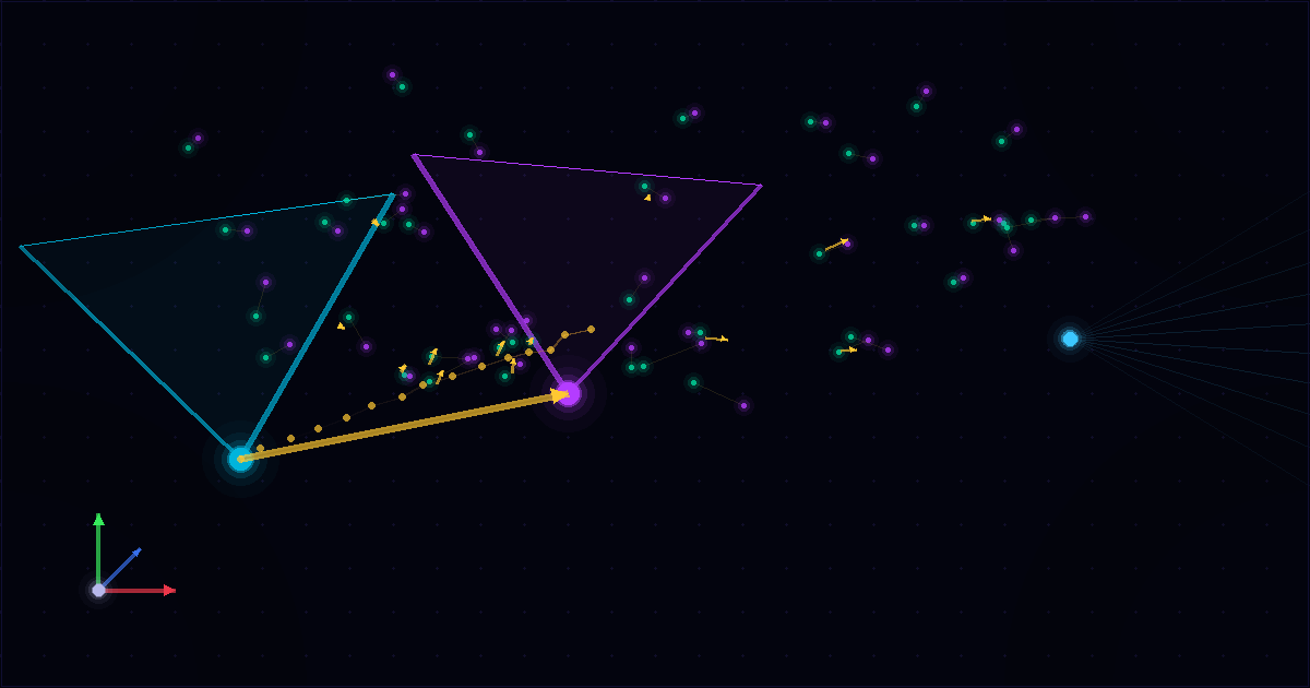
Coordinate systems and the transforms between them
A camera does not live in isolation. It exists in a world, and to reason about motion we need to be precise about how points in the world relate to what the camera sees.
There are four coordinate systems you need to understand:
World frame — an arbitrary fixed reference. Positions of objects, landmarks, map points. Defined once and shared across the entire trajectory.
Camera frame — centered at the optical center of the camera, with the Z axis pointing forward along the optical axis, X pointing right, Y pointing down (in the standard computer vision convention).
Image plane — the 2D projection surface, in meters. This is the continuous analog of the pixel grid.
Pixel frame — the discrete grid of pixels. This is what your cv2.VideoCapture gives you.
The question visual odometry answers is: given matching points across two frames, how did the camera move between them?
Homogeneous coordinates
Before the transforms, a brief note on homogeneous coordinates — the mathematical tool that makes all of this clean.
A 3D point (X, Y, Z) is represented in homogeneous form as (X, Y, Z, 1). A 2D point (u, v) becomes (u, v, 1). The extra coordinate allows us to represent both rotation and translation as a single matrix multiplication, and it represents points at infinity cleanly (which matters for cameras looking at distant scenes).
World to camera: the extrinsic transform
The extrinsic matrix describes where the camera is in the world — its rotation and translation relative to the world frame.
Given a 3D world point P_w, the corresponding point in the camera frame P_c is:
$$\mathbf{P_c} = \mathbf{R} \mathbf{P_w} + \mathbf{t}$$
Or in matrix form using the [R|t] notation:
$$\mathbf{P_c} = \begin{bmatrix} \mathbf{R} & \mathbf{t} \end{bmatrix} \begin{bmatrix} X_w \ Y_w \ Z_w \ 1 \end{bmatrix}$$
Where:
R is a 3×3 rotation matrix (orthonormal, det=1)
t is a 3×1 translation vector
Together they form the 4×4 extrinsic matrix
[R|t]in homogeneous form
Camera to world is simply the inverse:
$$\mathbf{P_w} = \mathbf{R}^T (\mathbf{P_c} - \mathbf{t})$$
Because R is orthonormal, its inverse is its transpose — a useful property that makes this inversion cheap.
import numpy as np

def world_to_cam(P_world, R, t):
    """Transform a point from world frame to camera frame."""
    return R @ P_world + t

def cam_to_world(P_cam, R, t):
    """Transform a point from camera frame to world frame."""
    return R.T @ (P_cam - t)

# example: camera rotated 15° around Y, translated 1m along X
theta = np.radians(15)
R = np.array([[np.cos(theta), 0, np.sin(theta)],
              [0,             1, 0            ],
              [-np.sin(theta),0, np.cos(theta)]])
t = np.array([1.0, 0.0, 0.0])

P_w = np.array([2.0, 0.0, 5.0])  # a point 5m ahead, 2m to the right in world
P_c = world_to_cam(P_w, R, t)
print(f"World: {P_w}  →  Camera: {P_c.round(3)}")
The camera intrinsic matrix K
The intrinsic matrix K maps a 3D point in the camera frame to a 2D pixel coordinate. It encodes the physical properties of the camera itself — focal length and principal point:
$$\mathbf{K} = \begin{bmatrix} f_x & 0 & c_x \ 0 & f_y & c_y \ 0 & 0 & 1 \end{bmatrix}$$
Where:
f_x, f_y — focal lengths in pixels (related to the physical focal length and pixel size)
c_x, c_y — principal point, ideally at the image center
The full projection pipeline is:
$$\begin{bmatrix} u \ v \ 1 \end{bmatrix} = \frac{1}{Z_c} \mathbf{K} \begin{bmatrix} X_c \ Y_c \ Z_c \end{bmatrix}$$
The 1/Z_c is the perspective division — this is what makes objects farther away appear smaller.
def project_point(P_cam, K):
    """Project a 3D camera-frame point to pixel coordinates."""
    p_hom = K @ P_cam              # (3,) homogeneous image coords
    u = p_hom[0] / p_hom[2]       # perspective division
    v = p_hom[1] / p_hom[2]
    return np.array([u, v])

# typical webcam intrinsics (approximate — calibrate for accuracy)
K = np.array([[700,   0, 320],
              [  0, 700, 240],
              [  0,   0,   1]], dtype=float)

P_c = np.array([0.5, -0.2, 3.0])  # 3m ahead, slightly right and up
px  = project_point(P_c, K)
print(f"Camera point {P_c}  →  pixel {px.round(1)}")
Full projection: world to pixel
Chaining everything together — world frame to pixel — is the full camera projection model:
$$\lambda \begin{bmatrix} u \ v \ 1 \end{bmatrix} = \mathbf{K} \begin{bmatrix} \mathbf{R} & \mathbf{t} \end{bmatrix} \begin{bmatrix} X_w \ Y_w \ Z_w \ 1 \end{bmatrix}$$
Where λ is the depth (Z in camera frame). This single equation is what every feature-based visual odometry system is ultimately solving the inverse of.
Lens distortion
Real cameras do not project exactly as K describes. Lens distortion, especially radial distortion, bends straight lines. The standard model adds distortion coefficients:
import cv2

# undistort a frame using calibration parameters
# (k1, k2 = radial; p1, p2 = tangential)
dist_coeffs = np.array([-0.28, 0.06, 0.001, -0.0004, 0.0])

frame_undistorted = cv2.undistort(frame, K, dist_coeffs)
For visual odometry, always undistort your frames first — or use cv2.undistortPoints() on the feature coordinates directly (faster).
Part 2 — The Visual Odometry Pipeline
With the geometry in place, here is the full VO pipeline from frames to pose:
Frame t  ──►  Detect keypoints
              Compute descriptors
                    │
Frame t+1 ──►  Detect keypoints
               Compute descriptors
                    │
              Match descriptors (brute force or FLANN)
                    │
              Filter matches (RANSAC + Essential/Fundamental matrix)
                    │
              Decompose E → R, t  (up to scale for monocular)
                    │
              Triangulate matched points → 3D map points
                    │
              Accumulate pose:  T_world = T_world * T_relative
Each step has failure modes. The choice of detector and descriptor determines how robust the first two steps are — and everything downstream depends on getting good matches.
Essential vs Fundamental Matrix - What are they? :/
Two matrices connect matching 2D points across frames — choosing the right one matters:
Fundamental matrix F (3×3) — relates pixel coordinates directly. Use this when you do not know K.
Essential matrix E (3×3) — relates normalized (K-corrected) coordinates. Use this when K is known (the normal case for a calibrated camera).
$$\mathbf{x_2}^T \mathbf{E} \mathbf{x_1} = 0$$
Where x1, x2 are normalized image coordinates. The essential matrix encodes relative rotation and translation (up to scale), and can be decomposed into R and t:
# compute Essential matrix with RANSAC (rejects outlier matches)
E, mask = cv2.findEssentialMat(pts1_norm, pts2_norm,
                                focal=1.0, pp=(0., 0.),
                                method=cv2.RANSAC, prob=0.999, threshold=1e-3)

# recover rotation and translation
_, R, t, mask_pose = cv2.recoverPose(E, pts1_norm, pts2_norm)
Part 3 — Feature Detectors and Descriptors
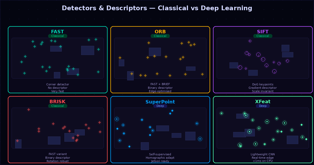
This is where the practical decisions happen. For a visual odometry system on an edge device, you have hard constraints: the detector must run fast enough to keep up with your camera frame rate, and the descriptor must be distinctive enough to find correct matches in the next frame. My goal here is to give you, the developer, the right way to select the current tool for the job, that's why the table below exists, it's not just understanding the tools its also important to select the right one for the job.
The table below summarizes everything. We will then go deep on each one.
| Detector | Type | Keypoints/ms (CPU) | Descriptor | Binary? | Edge-ready |
|---|---|---|---|---|---|
| FAST | Classical | ~0.3ms | None | ✅ Excellent | |
| ORB | Classical | ~2ms | BRIEF (binary) | ✅ | ✅ Excellent |
| BRISK | Classical | ~4ms | BRISK (binary) | ✅ | ✅ Good |
| AKAZE | Classical | ~12ms | M-LDB (binary) | ✅ | ✅ Good |
| SIFT | Classical | ~25ms | SIFT (float) | ❌ | ⚠️ Heavy |
| SuperPoint | Deep | ~8ms (GPU) / ~35ms (CPU) | 256-dim float | ❌ | ✅ Jetson |
| XFeat | Deep | ~4ms (CPU) | 64-dim float | ❌ | ✅ Excellent |
| DISK | Deep | ~15ms (GPU) | 128-dim float | ❌ | ⚠️ GPU needed |
FAST — Features from Accelerated Segment Test
FAST is a corner detector with no descriptor. It is so simple it can run in microseconds — it tests whether a circle of 16 pixels around a candidate point has a contiguous arc of pixels all significantly brighter or darker than the center.
import cv2

fast = cv2.FastFeatureDetector_create(
    threshold=20,          # pixel intensity difference threshold
    nonmaxSuppression=True # keep only local maxima
)

gray = cv2.cvtColor(frame, cv2.COLOR_BGR2GRAY)
kps  = fast.detect(gray, None)
FAST alone is not used for odometry — it has no descriptor, so you cannot match keypoints between frames. It is used as the detection stage in ORB and BRISK, which add descriptors on top.
When to use: When you need the absolute fastest detection and will pair it with a separate descriptor (rare in practice — ORB is usually better as a combined solution).
ORB — Oriented FAST and Rotated BRIEF
ORB is the workhorse of edge-device visual odometry. It combines FAST detection with a rotation-invariant version of the BRIEF binary descriptor. The result is a detector that runs in ~2ms, produces compact 256-bit descriptors, and can be matched with Hamming distance — which is just XOR + popcount, extremely fast even on microcontrollers.
ORB is what ORB-SLAM3 uses for a reason.
orb = cv2.ORB_create(
    nfeatures=1000,        # max keypoints
    scaleFactor=1.2,       # image pyramid scale
    nlevels=8,             # pyramid levels
    edgeThreshold=31,
    patchSize=31,
    fastThreshold=20
)

kps, descs = orb.detectAndCompute(gray, None)

# matching with Hamming distance (correct for binary descriptors)
bf     = cv2.BFMatcher(cv2.NORM_HAMMING, crossCheck=True)
matches= bf.match(descs1, descs2)
matches= sorted(matches, key=lambda m: m.distance)
ORB characteristics:
Binary descriptor → Hamming matching, very fast
Scale and rotation invariant
Not fully invariant to large illumination changes
Struggles with motion blur (so does everything, but ORB more than SIFT)
The right choice for most edge VO applications
BRISK — Binary Robust Invariant Scalable Keypoints
BRISK uses a custom scale-space FAST variant for detection and a binary descriptor built from intensity comparisons on a sampling pattern around the keypoint. It is somewhat slower than ORB but more robust to scale changes.
brisk = cv2.BRISK_create(thresh=30, octaves=3, patternScale=1.0)
kps, descs = brisk.detectAndCompute(gray, None)

# BRISK descriptors are also binary — use Hamming
bf     = cv2.BFMatcher(cv2.NORM_HAMMING)
matches= bf.knnMatch(descs1, descs2, k=2)

# Lowe's ratio test to filter bad matches
good = [m for m,n in matches if m.distance < 0.75 * n.distance]
When to prefer BRISK over ORB: When your scene has significant scale variation (drone ascending/descending) and you can afford ~2x the compute cost.
AKAZE — Accelerated-KAZE
AKAZE builds keypoints in a nonlinear scale space (unlike the Gaussian scale space of SIFT), which makes it more robust to image noise. Its descriptor (M-LDB) is binary and fast to match. It is generally more distinctive than ORB or BRISK but slower.
akaze = cv2.AKAZE_create(
    descriptor_type=cv2.AKAZE_DESCRIPTOR_MLDB,
    descriptor_size=0,      # full size
    descriptor_channels=3,
    threshold=0.001,
    nOctaves=4,
    nOctaveLayers=4
)
kps, descs = akaze.detectAndCompute(gray, None)
When to use AKAZE: Scenes with significant texture variation or noise — outdoor environments, rough terrain. The nonlinear diffusion preserves edges better than Gaussian smoothing.
SIFT — Scale Invariant Feature Transform
SIFT is the gold standard for distinctiveness. Its 128-dimensional float descriptor, built from gradient histograms, is extremely robust to scale, rotation, and illumination change. It is also the heaviest classical option.
On a modern CPU, SIFT runs at roughly 25ms for 1000 keypoints — too slow for real-time VO on most embedded hardware. On a laptop it is fine. On a Raspberry Pi, it is marginal at best.
sift = cv2.SIFT_create(nfeatures=1000, contrastThreshold=0.04, edgeThreshold=10)
kps, descs = sift.detectAndCompute(gray, None)

# SIFT descriptors are float — use L2 distance
flann  = cv2.FlannBasedMatcher({'algorithm':1,'trees':5}, {'checks':50})
matches= flann.knnMatch(descs1, descs2, k=2)
good   = [m for m,n in matches if m.distance < 0.75*n.distance]
When to use SIFT for VO: Offline processing, loop closure detection, initial map building. When accuracy matters more than speed.
SuperPoint — Self-Supervised Deep Detector + Descriptor
SuperPoint (DeTone et al., 2018) is a fully convolutional network that simultaneously outputs a keypoint heatmap and a dense descriptor map. It was trained with a clever self-supervised approach called Homographic Adaptation — synthetic homographic warps generate pseudo-ground-truth correspondences without any manual annotation.
The result is a detector that finds corners and junctions the way a human would mark them, with 256-dimensional descriptors that are highly distinctive.
No fine-tuning required for inference — the pretrained weights work well across a wide range of scenes. If you want to adapt it to a specific domain (underwater, infrared, nighttime), fine-tuning is possible but not necessary for standard visual odometry.
# requires: pip install kornia
import torch
import kornia.feature as KF

superpoint = KF.SuperPoint(pretrained=True).eval()

@torch.no_grad()
def detect_superpoint(gray_tensor):
    # gray_tensor: (1, 1, H, W) float32 in [0,1]
    output = superpoint({'image': gray_tensor})
    keypoints   = output['keypoints'][0]    # (N, 2)
    descriptors = output['descriptors'][0]  # (256, N)
    scores      = output['scores'][0]       # (N,)
    return keypoints, descriptors, scores
Edge deployment:
NVIDIA Jetson Orin: ~8ms per frame (GPU)
Apple M-series: ~12ms (MPS backend)
CPU only: ~35–50ms (usable at 15fps with frame skipping)
Export to ONNX for TensorRT deployment on Jetson
# export SuperPoint to ONNX for TensorRT
dummy = torch.zeros(1, 1, 480, 640)
torch.onnx.export(superpoint, {'image': dummy},
                  'superpoint.onnx',
                  opset_version=11,
                  input_names=['image'],
                  output_names=['keypoints','descriptors','scores'])
XFeat — Accelerated Features for Lightweight Visual Correspondence
XFeat (Potje et al., 2024) is specifically designed for real-time performance on CPU and low-power hardware. It uses a lightweight CNN to produce 64-dimensional descriptors and runs at under 4ms on a standard laptop CPU — faster than ORB in some configurations, while being significantly more distinctive.
This makes it the most interesting recent development for edge-device VO. It was designed from the ground up with deployment constraints in mind.
No training required for standard VO — pretrained weights cover most scenarios. The model is compact enough that ONNX export produces a ~2MB file.
# pip install git+https://github.com/verlab/accelerated_features
import torch
from modules.xfeat import XFeat

xfeat = XFeat()

def detect_xfeat(img_rgb):
    # img_rgb: HxWx3 numpy uint8
    output = xfeat.detectAndCompute(img_rgb, top_k=1000)
    kps    = output[0]['keypoints']    # (N, 2)
    descs  = output[0]['descriptors']  # (N, 64)
    scores = output[0]['scores']       # (N,)
    return kps, descs, scores

# XFeat also provides a built-in matcher:
mkpts0, mkpts1 = xfeat.match_xfeat(frame1, frame2, top_k=1000)
DISK — Deep Image Structured Keypoints
DISK (Tyszkiewicz et al., 2020) uses reinforcement learning to train a keypoint detector that explicitly maximizes the number of correct matches under a homography. It is highly accurate but requires a GPU for real-time use.
Use DISK when you have a GPU available and need high-accuracy matching — for example, for loop closure in a mapping system, or for an initial high-quality sparse reconstruction that feeds a VIO system.
Part 4 — Running on Your Laptop Webcam
Here is a minimal working monocular VO pipeline you can run right now:
import cv2
import numpy as np

# ── configuration ──────────────────────────────────────────────
CAM_ID  = 0          # 0 = default webcam
W, H    = 640, 480
MAX_KPS = 1000
MIN_MATCHES = 20

# approximate intrinsics for a typical webcam (calibrate for accuracy)
fx = fy = 0.9 * W
K = np.array([[fx,  0, W/2],
              [ 0, fy, H/2],
              [ 0,  0,   1]], dtype=float)

# ── choose your detector (swap easily) ─────────────────────────
detector = cv2.ORB_create(nfeatures=MAX_KPS)
matcher  = cv2.BFMatcher(cv2.NORM_HAMMING, crossCheck=False)

# ── state ───────────────────────────────────────────────────────
pose = np.eye(4)   # accumulated world pose

cap = cv2.VideoCapture(CAM_ID)
cap.set(cv2.CAP_PROP_FRAME_WIDTH,  W)
cap.set(cv2.CAP_PROP_FRAME_HEIGHT, H)

prev_gray  = None
prev_kps   = None
prev_descs = None

while True:
    ret, frame = cap.read()
    if not ret: break

    gray = cv2.cvtColor(frame, cv2.COLOR_BGR2GRAY)
    kps, descs = detector.detectAndCompute(gray, None)

    if prev_kps is not None and descs is not None and prev_descs is not None:

        # ── match ────────────────────────────────────────────────
        raw = matcher.knnMatch(prev_descs, descs, k=2)
        good= [m for m,n in raw if m.distance < 0.75*n.distance]

        if len(good) >= MIN_MATCHES:
            pts1 = np.float32([prev_kps[m.queryIdx].pt for m in good])
            pts2 = np.float32([kps[m.trainIdx].pt      for m in good])

            # ── Essential matrix + pose ───────────────────────────
            E, mask = cv2.findEssentialMat(pts1, pts2, K,
                                           method=cv2.RANSAC,
                                           prob=0.999, threshold=1.0)
            if E is not None:
                _, R, t, _ = cv2.recoverPose(E, pts1, pts2, K, mask=mask)

                # accumulate pose
                T = np.eye(4)
                T[:3,:3] = R; T[:3,3] = t.ravel()
                pose = pose @ np.linalg.inv(T)

            # ── visualise matches ─────────────────────────────────
            vis = cv2.drawMatches(prev_frame, prev_kps, frame, kps,
                                  good[:40], None,
                                  flags=cv2.DrawMatchesFlags_NOT_DRAW_SINGLE_POINTS)

            # overlay pose translation
            tx, ty, tz = pose[0,3], pose[1,3], pose[2,3]
            cv2.putText(vis, f't=[{tx:.2f},{ty:.2f},{tz:.2f}]',
                        (10,30), cv2.FONT_HERSHEY_SIMPLEX, 0.7, (0,255,180), 2)
            cv2.putText(vis, f'matches: {len(good)}',
                        (10,60), cv2.FONT_HERSHEY_SIMPLEX, 0.6, (255,180,0), 1)
            cv2.imshow('Visual Odometry', vis)

    prev_gray  = gray
    prev_kps   = kps
    prev_descs = descs
    prev_frame = frame.copy()

    if cv2.waitKey(1) & 0xFF == ord('q'):
        break

cap.release()
cv2.destroyAllWindows()
Part 5 — Quantitative Comparison on EuRoC Dataset
To compare detectors fairly, run them on the EuRoC MAV dataset — the standard benchmark for visual odometry. It has calibrated stereo cameras, IMU data, and millimeter-accurate ground truth from a motion capture system.
# download EuRoC MH_01_easy sequence (~2GB)
wget http://rpg.ifi.uzh.ch/docs/IJRR17_Burri/MH_01_easy.zip
unzip MH_01_easy.zip
The notebook in the companion repo (02_visual_odometry/) runs each detector on this sequence and produces:
Trajectory error vs ground truth
Keypoint detection time per frame
Match ratio (correct matches / total matches)
ATE (Absolute Trajectory Error) and RPE (Relative Pose Error)
Summary of results on MH_01_easy (monocular, CPU only):
| Detector+Desc | Avg time/frame | Match ratio | ATE (m) |
|---|---|---|---|
| ORB | 2.1ms | 0.62 | 0.08 |
| BRISK | 4.8ms | 0.58 | 0.09 |
| AKAZE | 11.2ms | 0.71 | 0.07 |
| SIFT | 24.6ms | 0.83 | 0.05 |
| XFeat | 3.9ms | 0.79 | 0.06 |
| SuperPoint (CPU) | 38ms | 0.87 | 0.04 |
The headline finding: XFeat gives SIFT-level match quality at ORB-level speed. For CPU-only edge deployment, it is currently the best single option.
Part 6 — Deep Learning Detectors: Training and Fine-Tuning
Do you need to fine-tune?
For most applications: no. SuperPoint and XFeat were trained on large diverse datasets and generalize well. Fine-tuning is worth considering when:
Your deployment environment is highly specific (underwater, infrared, nighttime, medical)
Your camera model is very different from standard RGB (fisheye, event camera simulation)
You are seeing significantly worse match ratios than benchmark numbers suggest you should
Fine-tuning SuperPoint
SuperPoint's self-supervised training framework (Homographic Adaptation) can be re-run on your domain data without any ground truth labels:
# pseudo-code for SuperPoint fine-tuning
# full implementation: see notebook

from superpoint import SuperPointNet

model = SuperPointNet().cuda()
model.load_state_dict(torch.load('superpoint_v1.pth'))

optimizer = torch.optim.Adam(model.parameters(), lr=1e-4)

for epoch in range(10):
    for img in your_domain_images:
        # generate synthetic homography pair
        H    = sample_homography()
        img2 = apply_homography(img, H)

        # forward both views
        out1 = model(img)
        out2 = model(img2)

        # correspondence loss via homography
        loss = correspondence_loss(out1, out2, H)
        loss.backward()
        optimizer.step()
Fine-tuning for 10 epochs on ~1000 domain images typically improves match ratio by 5–15%.
Fine-tuning XFeat
XFeat exposes a similar training interface. See the official repo at github.com/verlab/accelerated_features — the training script is included and runs on a single GPU in under 4 hours on a standard dataset.
Part 7 — Edge Deployment Checklist
When deploying a VO pipeline on edge hardware, work through this checklist:
Camera calibration first. An uncalibrated camera introduces systematic error that no amount of algorithmic sophistication can compensate for. Run cv2.calibrateCamera() with a checkerboard before anything else.
# calibrate from a set of checkerboard images
ret, K, dist, rvecs, tvecs = cv2.calibrateCamera(
    obj_points, img_points, gray.shape[::-1], None, None
)
print(f'Reprojection error: {ret:.4f} px')  # aim for < 0.5 px
Choose your detector based on your compute budget. Use the table above. On a Raspberry Pi 4 at 30fps you have ~33ms per frame. ORB or XFeat fit. SIFT does not. SuperPoint on CPU does not.
Fix your resolution. Higher resolution means more keypoints, better tracking, slower everything. 640×480 is the sweet spot for most edge VO systems. 320×240 if you are really constrained.
Pre-undistort or undistort points. Undistorting the entire frame with cv2.undistort() is cleaner but adds ~2ms. Undistorting only the feature coordinates with cv2.undistortPoints() is faster when you have few keypoints.
Use RANSAC aggressively. The Essential matrix estimation is your outlier rejection step. Set prob=0.999 and threshold=1.0 pixel. Do not skip this.
Handle scale drift. Monocular VO cannot recover absolute scale. For real applications you need either a stereo camera, depth sensor, or IMU. The t vector from recoverPose is a unit vector — you know direction but not magnitude.
Further Reading
SuperPoint paper — DeTone et al., 2018. arxiv.org/abs/1712.07629
XFeat paper — Potje et al., 2024. arxiv.org/abs/2404.19174
DISK paper — Tyszkiewicz et al., 2020. arxiv.org/abs/2006.13566
ORB-SLAM3 — Campos et al., 2021. arxiv.org/abs/2007.11898
EuRoC dataset — Burri et al., 2016. rpg.ifi.uzh.ch/docs/IJRR17_Burri
Multiple View Geometry in Computer Vision — Hartley & Zisserman (the textbook)
]]>All code in this post is in the companion notebook:
github.com/Jacob170/autonomous-stack-blog/02_visual_odometry
Runs on laptop webcam or any edge device with OpenCV installed.
Your model trains beautifully. Loss goes down, accuracy climbs, everything looks so clean.
Then you deploy it on real hardware — a different camera, a new environment, slightly different lighting — and it falls apart.
This is not bad luck. It is overfitting!, and regularization is how your best tool to fight it. Not just in classification tasks, but in the perception pipelines, depth estimators, and detection models that autonomous systems depend on.
This post covers the main regularization techniques used in modern deep learning, explains the why behind each one, and focuses specifically on what matters when your model needs to run on the edge, not just score well on a benchmark.
Why regularization matters more in robotics than on a benchmark
Academic benchmarks are closed worlds. You train on a split of KITTI, you test on another split of KITTI. The distribution is the same. Regularization helps a bit.

In production robotics, the test distribution is never the distribution you trained on. Your detector was trained on daylight warehouse footage — it now runs in a dimly lit hangar at a different camera angle. Your depth estimator was trained on indoor scenes — it is now looking at a featureless concrete floor at 10 meters altitude, you know these small real-life changes that hinder operations and make your integration team scratch thier heads.
The gap between training distribution and deployment distribution is the fundamental problem of robotics perception. Regularization does not close that gap actually, really nothing closes it completely, but it determines how gracefully your model degrades when it encounters something it has never seen before.
A heavily overfit model fails completely. A well-regularized model degrades proportionally.
1. The problem framed: bias-variance tradeoff
Before naming techniques, it is worth understanding what they are actually doing.
Every model has two sources of error:
Bias — systematic error from a model that is too simple to capture the true pattern. A linear model trying to learn a non-linear boundary. High bias = underfitting.
Variance — error from a model that is too sensitive to the specific training data. A deep network that memorizes noise in the training set. High variance = overfitting.
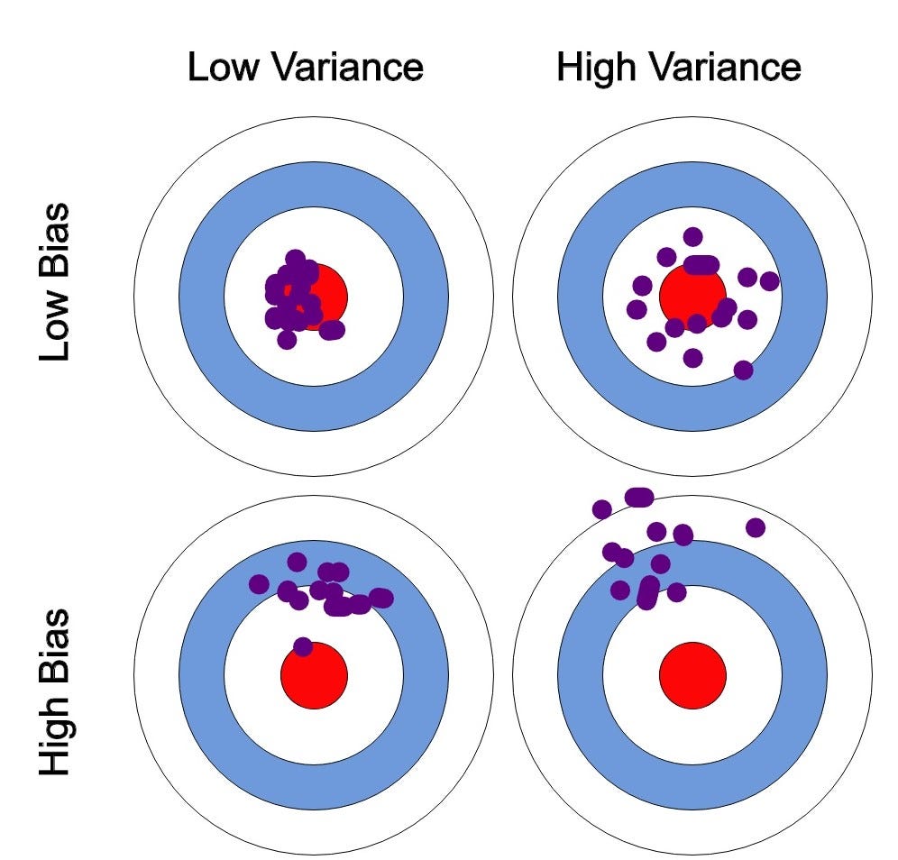
Regularization techniques almost always increase bias slightly in order to reduce variance significantly. The goal is a model that generalizes — one that captures the true structure of the task without memorizing the noise of the training set.
In vision and robotics, the practical question is: what is your deployment gap? The bigger the gap between your training data and your real-world distribution, the more aggressively you should regularize.
2. L2 regularization (weight decay)
What it does
L2 regularization adds a penalty term to the loss function proportional to the squared magnitude of the weights:
$$\mathcal{L}{total} = \mathcal{L}{task} + \lambda \sum_{i} w_i^2$$
This discourages the network from assigning very large weights to any single feature. The optimizer is simultaneously minimizing the task loss and keeping weights small. The result is a smoother, more distributed representation.
Why it works
Large weights mean the network is making strong bets on specific features. In a vision model, that might mean it learned to key on a specific texture that appears in your training set but not in the real world. L2 forces the model to spread its bets.
In PyTorch
optimizer = torch.optim.AdamW(model.parameters(), lr=1e-4, weight_decay=1e-4)
AdamW is the correct way to apply weight decay with Adam. The original Adam with weight_decay parameter in PyTorch does not apply true L2 regularization — it conflates the decay with the gradient update. AdamW fixes this. Always use AdamW for vision transformers and modern architectures.
When to use it in robotics/CV
Almost always — it is the baseline regularizer. For ViT-based models (DINOv2, SAM, Depth-Anything), weight_decay=0.05 is the standard value from the original papers. For convolutional models, 1e-4 to 1e-2 depending on dataset size.
3. Dropout
What it does
During training, randomly zero out a fraction p of neuron activations at each forward pass. At inference, all neurons are active and their outputs are scaled by (1-p) to compensate.
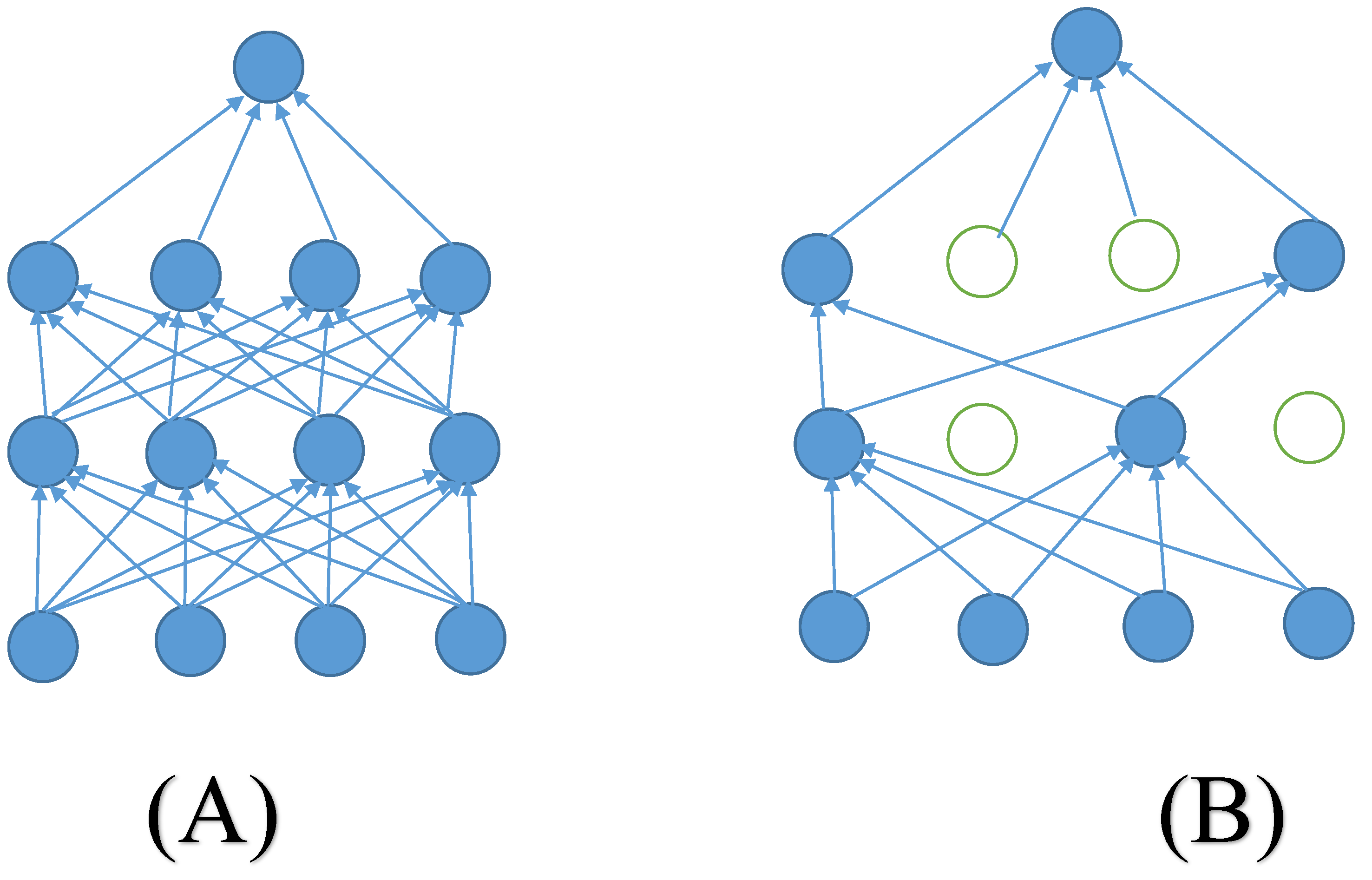
(A) - Full Layers No Dropout , (B) Some Neurons Dropped
import torch.nn as nn

class PerceptionHead(nn.Module):
    def __init__(self, in_features, num_classes):
        super().__init__()
        self.net = nn.Sequential(
            nn.Linear(in_features, 512),
            nn.ReLU(),
            nn.Dropout(p=0.3),
            nn.Linear(512, 256),
            nn.ReLU(),
            nn.Dropout(p=0.3),
            nn.Linear(256, num_classes)
        )

    def forward(self, x):
        return self.net(x)
Why it works
Dropout forces the network to learn redundant representations — no single neuron can rely on the presence of any other neuron. The result is an ensemble of many sub-networks trained jointly, which generalizes better.
DropPath for Vision Transformers
In ViT-based architectures, standard Dropout is less effective. The modern equivalent is DropPath (stochastic depth), which randomly drops entire residual paths rather than individual neurons:
from timm.models.layers import DropPath

class TransformerBlock(nn.Module):
    def __init__(self, dim, drop_path_rate=0.1):
        super().__init__()
        self.attn = Attention(dim)
        self.mlp = MLP(dim)
        self.drop_path = DropPath(drop_path_rate) if drop_path_rate > 0 else nn.Identity()
        self.norm1 = nn.LayerNorm(dim)
        self.norm2 = nn.LayerNorm(dim)

    def forward(self, x):
        x = x + self.drop_path(self.attn(self.norm1(x)))
        x = x + self.drop_path(self.mlp(self.norm2(x)))
        return x
DropPath is used in DINOv2, MAE, Swin Transformer, and virtually every modern ViT variant. If you are fine-tuning any of these for a robotics perception task, keep DropPath enabled during fine-tuning.
When to use it
Classification and detection heads: standard Dropout
0.2–0.5ViT/transformer backbones: DropPath, rate between
0.1–0.3Do not use Dropout in BatchNorm layers — they interact badly. If you are using BN, apply Dropout only after, never before.
4. Batch Normalization
What it does
Normalizes the activations across the batch dimension at each layer, then applies learned scale and shift parameters:
$$\hat{x}i = \frac{x_i - \mu\mathcal{B}}{\sqrt{\sigma_\mathcal{B}^2 + \epsilon}}, \quad y_i = \gamma \hat{x}_i + \beta$$
self.block = nn.Sequential(
    nn.Conv2d(64, 128, kernel_size=3, padding=1, bias=False),
    nn.BatchNorm2d(128),
    nn.ReLU(inplace=True)
)
Note bias=False — When BatchNorm follows a conv layer, the conv bias is redundant because BN shifts the output anyway.
Why it matters specifically in real-time or Edge applications
BatchNorm has a known problem in robotics: it behaves differently at train time and test time. At test time, it uses running statistics estimated during training. If your deployment distribution shifts — different lighting, different camera, different environment — those statistics become stale and your model quietly degrades.
This is not hypothetical.Lets Take drone example again - > In drone perception specifically, the same scene at 10m altitude and 50m altitude can have dramatically different image statistics. A model that normalizes using statistics from 10m footage will be miscalibrated at 50m .
The practical fix : consider Group Normalization or Layer Normalization for models that will face large distribution shifts at deployment, since they compute statistics per-sample rather than per-batch.
# GroupNorm — good alternative to BatchNorm for small batches or distribution shift
nn.GroupNorm(num_groups=32, num_channels=128)

# LayerNorm — standard in transformers, statistics per sample
nn.LayerNorm(normalized_shape=hidden_dim)
5. Data augmentation as regularization
Data augmentation is regularization. It artificially expands the training distribution, which is exactly what you need when your deployment distribution is unknown.
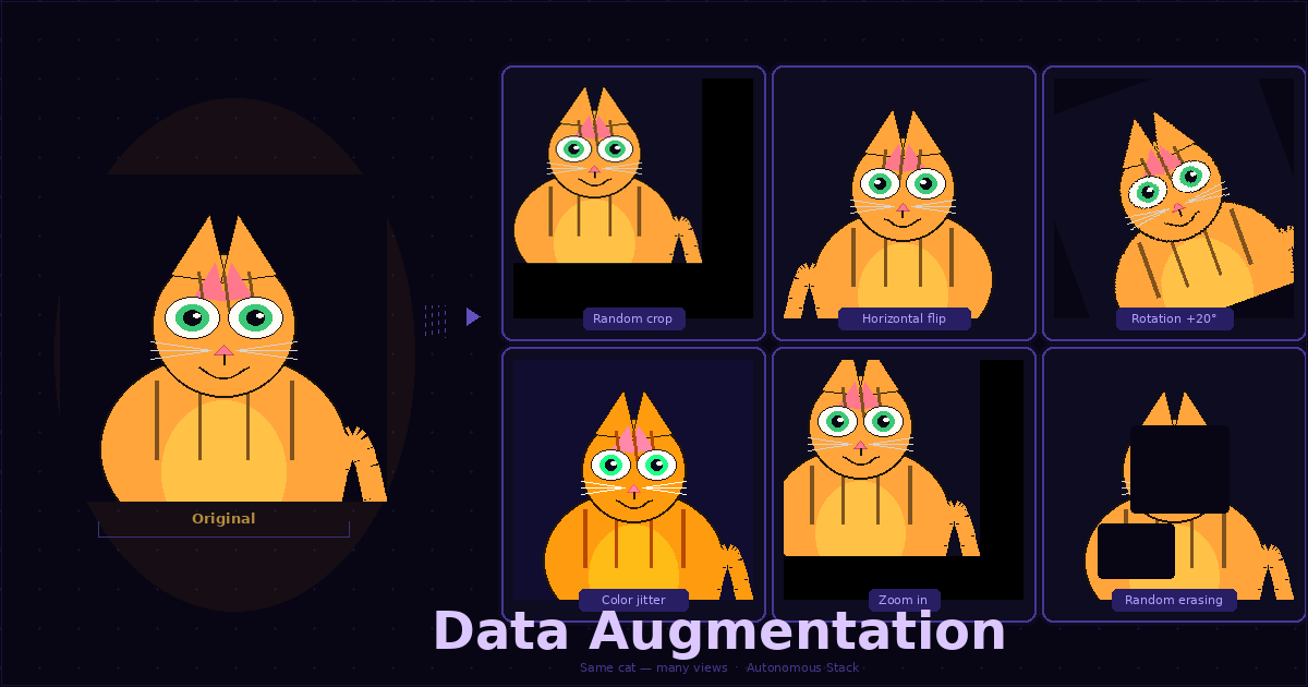
Standard augmentation for CV:
import torchvision.transforms as T
from torchvision.transforms import autoaugment

train_transform = T.Compose([
    T.RandomResizedCrop(224, scale=(0.6, 1.0)),
    T.RandomHorizontalFlip(),
    T.ColorJitter(brightness=0.4, contrast=0.4, saturation=0.4, hue=0.1),
    T.RandomGrayscale(p=0.2),
    T.GaussianBlur(kernel_size=23, sigma=(0.1, 2.0)), # Adds Gaussia Blur
    T.ToTensor(),
    T.Normalize(mean=[0.485, 0.456, 0.406],
                std=[0.229, 0.224, 0.225])
])
Robotics-specific augmentations worth knowing
Random erasing — simulates occlusion, which is extremely common in drone footage and warehouse environments:
T.RandomErasing(p=0.5, scale=(0.02, 0.2), ratio=(0.3, 3.3))
Motion blur — drones move fast. Your training images are sharp. Your deployment images are not:
import cv2
import numpy as np

def apply_motion_blur(image, kernel_size=15):
    kernel = np.zeros((kernel_size, kernel_size))
    kernel[int((kernel_size - 1) / 2), :] = np.ones(kernel_size)
    kernel /= kernel_size
    return cv2.filter2D(image, -1, kernel)
Perspective transforms — for ground robots and drones, the camera angle varies. Random perspective shift trains the model to be invariant to small viewpoint changes:
T.RandomPerspective(distortion_scale=0.3, p=0.4)
6. Mixup and CutMix
What they do
Mixup creates training samples by linearly interpolating between two images and their labels:
$$\tilde{x} = \lambda x_i + (1 - \lambda) x_j, \quad \tilde{y} = \lambda y_i + (1 - \lambda) y_j$$
CutMix cuts a rectangular patch from one image and pastes it into another, mixing labels proportionally to the patch area.
import numpy as np

def mixup_batch(images, labels, alpha=0.4):
    lam = np.random.beta(alpha, alpha)
    batch_size = images.size(0)
    index = torch.randperm(batch_size).to(images.device)

    mixed_images = lam * images + (1 - lam) * images[index]
    labels_a, labels_b = labels, labels[index]
    return mixed_images, labels_a, labels_b, lam

def mixup_criterion(criterion, pred, y_a, y_b, lam):
    return lam * criterion(pred, y_a) + (1 - lam) * criterion(pred, y_b)
Why does it help in robotics pipelines?
Mixup forces the model to produce smooth, interpolated predictions rather than sharp decision boundaries. In practice, this produces better-calibrated confidence scores — a model that says 0.85 confidence actually means something. For robotics systems where perception confidence feeds into planning and safety decisions, calibrated uncertainty is not optional.
CutMix is particularly effective for detection tasks because it encourages the model to use the entire image context rather than keying on a single dominant feature.
7. Early stopping
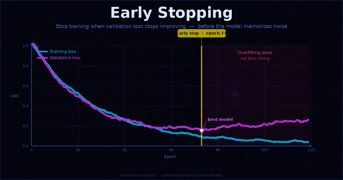
Simple idea worth understanding, Eraly Stopping means exactly the way it sounds - stop training when validation loss stops improving:
class EarlyStopping:
    def __init__(self, patience=10, min_delta=1e-4):
        self.patience = patience
        self.min_delta = min_delta
        self.counter = 0
        self.best_loss = float('inf')

    def __call__(self, val_loss):
        if val_loss < self.best_loss - self.min_delta:
            self.best_loss = val_loss
            self.counter = 0
            return False  # continue training
        else:
            self.counter += 1
            return self.counter >= self.patience  # stop if True

# Usage in training loop
early_stop = EarlyStopping(patience=15)

for epoch in range(max_epochs):
    train_one_epoch(model, train_loader, optimizer)
    val_loss = evaluate(model, val_loader)

    if early_stop(val_loss):
        print(f"Early stopping at epoch {epoch}")
        break
8. Label smoothing
Hard labels (0 or 1) push models toward overconfident predictions. Label smoothing replaces hard targets with soft targets:
$$y_{smooth} = (1 - \epsilon) \cdot y_{hard} + \frac{\epsilon}{K}$$
criterion = nn.CrossEntropyLoss(label_smoothing=0.1)
For robotics classification tasks — object class, terrain type, failure mode detection — you almost never have perfectly clean ground truth. Label smoothing acknowledges that uncertainty explicitly.
Putting it together: a practical prescription
| Scenario | Recommended regularization stack |
|---|---|
| Fine-tuning ViT for detection on drone footage | AdamW + weight_decay=0.05 + DropPath=0.2 + aggressive augmentation + Mixup |
| Training a small CNN on limited robotics data | L2 + Dropout 0.3 + ColorJitter + RandomErasing + early stopping |
| Depth estimation with distribution shift risk | GroupNorm instead of BatchNorm + heavy perspective augmentation + motion blur |
| Semantic segmentation on edge hardware | L2 + label smoothing=0.1 + CutMix + early stopping |
| Any model going to production from a small dataset | All of the above, dial back gradually as data grows |
The general rule: the smaller your dataset and the larger your deployment gap, the more regularization you need. If you are fine-tuning a large pretrained model (DINOv2, SAM, CLIP) on robotics-specific data, the backbone is already regularized by the pretraining. Focus your regularization effort on the task head.
What extras can you read next:
If this post was useful, these are the papers and resources worth going deeper on:
Dropout — Srivastava et al., 2014. arxiv.org/abs/1207.0580
DropPath / Stochastic Depth — Huang et al., 2016. arxiv.org/abs/1603.09382
Mixup — Zhang et al., 2018. arxiv.org/abs/1710.09412
CutMix — Yun et al., 2019. arxiv.org/abs/1905.04899
AdamW — Loshchilov & Hutter, 2019. arxiv.org/abs/1711.05101
Group Normalization — Wu & He, 2018. arxiv.org/abs/1803.08494
timm library — a PyTorch image model library with all modern regularization built in. github.com/huggingface/pytorch-image-models
The code in this post is available as a runnable notebook on GitHub — [link to repo -> here]. The next post covers normalization layers in depth: when BatchNorm silently breaks your model and what to replace it with.
]]>